How To Open Rstudio After Installation

Tutorial: Getting Started with R and RStudio

Published: August 5, 2022

In this tutorial we'll acquire how to begin programming with R using RStudio. We'll install R, and RStudio RStudio, an extremely pop development environment for R. We'll learn the primal RStudio features in order to start programming in R on our own.

If you lot already know how to apply RStudio and want to learn some tips, tricks, and shortcuts, cheque out this Dataquest blog mail.

Table of Contents

• 1. Install R
• 2. Install RStudio
• 3. Starting time Await at RStudio
• four. The Console
• 5. The Global Environment
• half dozen. Install thetidyverse Packages
• seven. Load thetidyverse Packages into Retentiveness
• 8. Place Loaded Packages
• 9. Get Help on a Package
• 10. Become Help on a Function
• 11. RStudio Projects
• 12. Save Your "Real" Piece of work. Delete the Rest.
• 13. R Scripts
• 14. Run Code
• 15. Access Congenital-in Datasets
• xvi. Way
• 17. Reproducible Reports with R Markdown
• 18. Utilize RStudio Deject
• xix. Get Your Hands Muddy!
• Boosted Resource
• Bonus: Cheatsheets

Getting Started with RStudio

RStudio is an open-source tool for programming in R. RStudio is a flexible tool that helps y'all create readable analyses, and keeps your code, images, comments, and plots together in one place. It'due south worth knowing about the capabilities of RStudio for data assay and programming in R.

Using RStudio for information assay and programming in R provides many advantages. Here are a few examples of what RStudio provides:

• An intuitive interface that lets us keep runway of saved objects, scripts, and figures
• A text editor with features like color-coded syntax that helps united states of america write clean scripts
• Car complete features save time
• Tools for creating documents containing a projection's code, notes, and visuals
• Dedicated Project folders to continue everything in one place

RStudio can besides exist used to plan in other languages including SQL, Python, and Bash, to name a few.

Only before we can install RStudio, we'll need to accept a recent version of R installed on our computer.

1. Install R

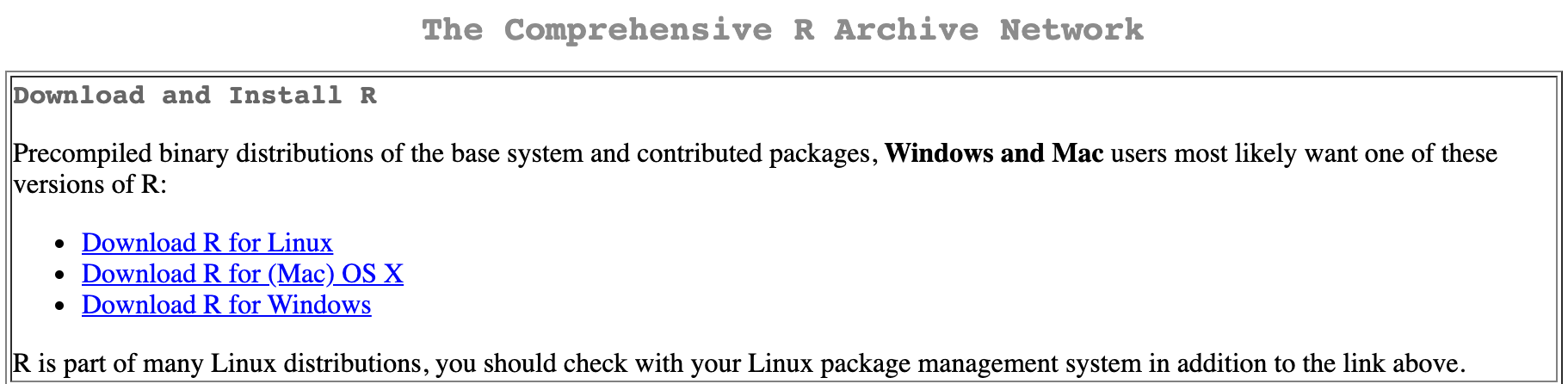
R is bachelor to download from the official R website. Await for this department of the web page:

The version of R to download depends on our operating system. Beneath, we include installation instructions for Mac Os X, Windows, and Linux (Ubuntu).

MAC Os X

• Select the Download R for (Mac) OSX option.
• Look for the near up-to-date version of R (new versions are released ofttimes and announced toward the tiptop of the page) and click the .pkg file to download.
• Open the .pkg file and follow the standard instructions for installing applications on MAC OS Ten.
• Drag and drib the R application into the Applications folder.

Windows

• Select the Download R for Windows option.
• Select base, since this is our first installation of R on our figurer.
• Follow the standard instructions for installing programs for Windows. If we are asked to select Customize Startup or Accept Default Startup Options, choose the default options.

Linux/Ubuntu

• Select the Download R for Linux option.
• Select the Ubuntu option.
• Alternatively, select the Linux package management organization relevant to y'all if you are non using Ubuntu.

RStudio is compatible with many versions of R (R version 3.0.ane or newer equally of July, 2022). Installing R separately from RStudio enables the user to select the version of R that fits their needs.

two. Install RStudio

At present that R is installed, we tin install RStudio. Navigate to the RStudio downloads page.

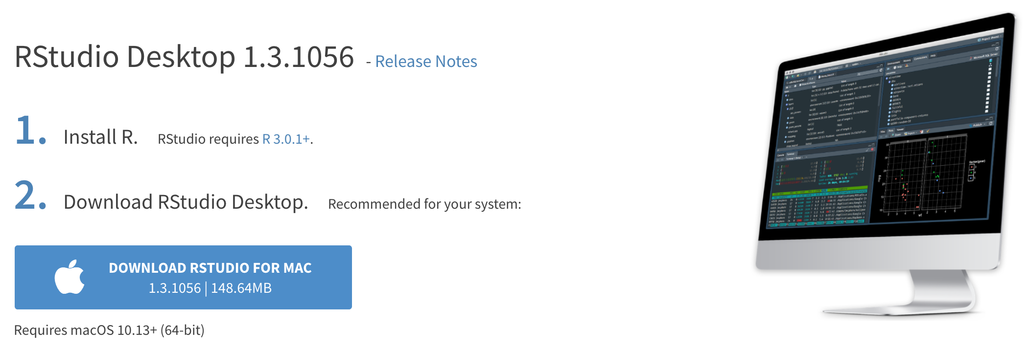
When nosotros accomplish the RStudio downloads page, let's click the "Download" button of the RStudio Desktop Open Source License Free selection:

Our operating system is usually detected automatically and then we can directly download the correct version for our computer by clicking the "Download RStudio" button. If we want to download RStudio for some other operating system (other than the one nosotros are running), navigate down to the "All installers" section of the folio.

iii. First Await at RStudio

When nosotros open up RStudio for the get-go time, we'll probably see a layout like this:

Only the groundwork colour will be white, and then don't expect to see this blueish-colored background the first time RStudio is launched. Check out this Dataquest web log to learn how to customize the appearance of RStudio.

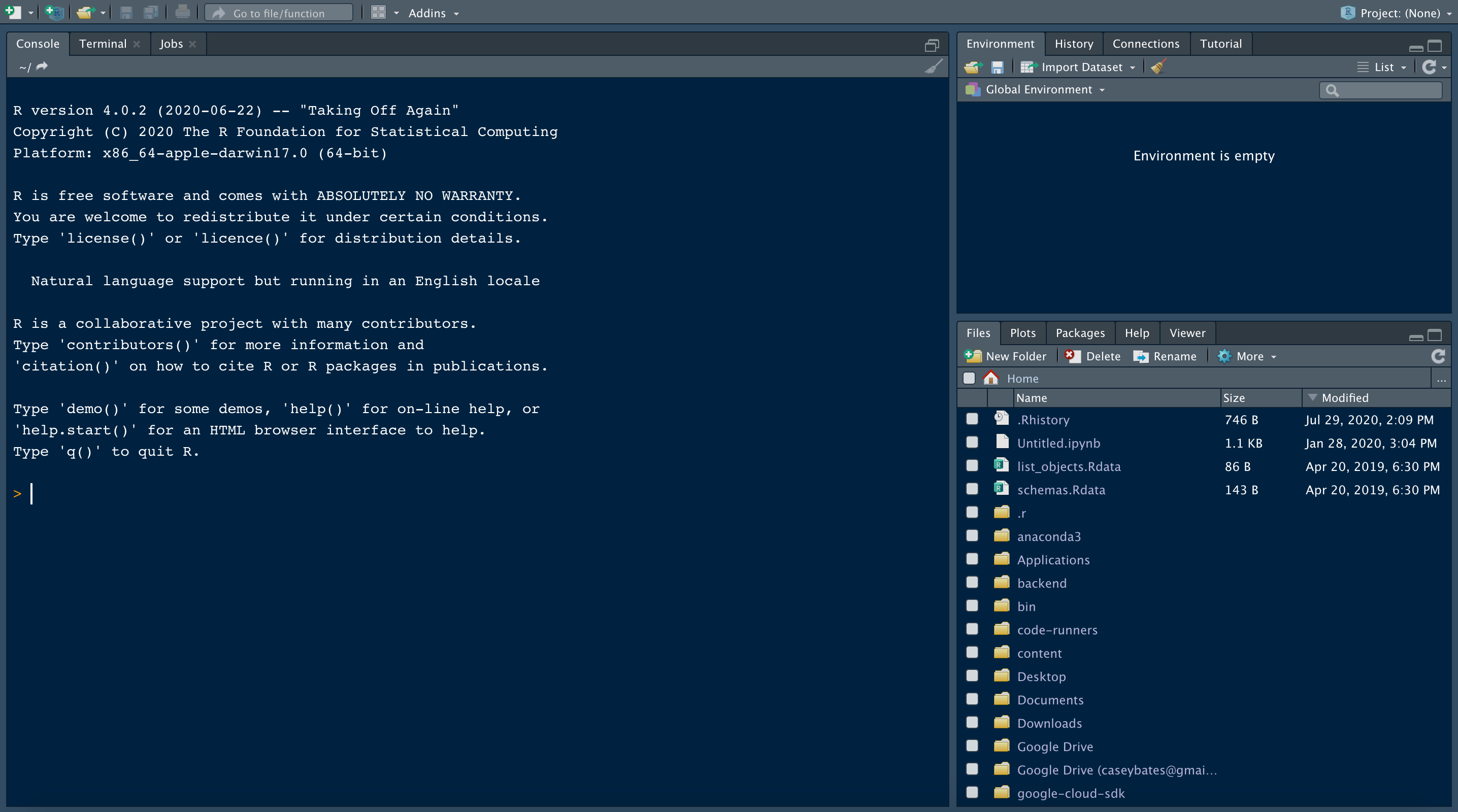
When we open RStudio, R is launched too. A common mistake by new users is to open R instead of RStudio. To open up RStudio, search for RStudio on the desktop, and pivot the RStudio icon to the preferred location (east.thousand. Desktop or toolbar).

4. The Console

Let's beginning off by introducing some features of the Panel. The Console is a tab in RStudio where we can run R code.

Notice that the window pane where the console is located contains iii tabs: Console, Terminal and Jobs (this may vary depending on the version of RStudio in use). We'll focus on the Console for now.

When we open RStudio, the panel contains information about the version of R we're working with. Scroll down, and attempt typing a few expressions similar this i. Printing the enter key to see the upshot.

            one + ii          

Equally we tin come across, we tin can use the console to exam code immediately. When we type an expression like i + 2, we'll see the output below later striking the enter key.

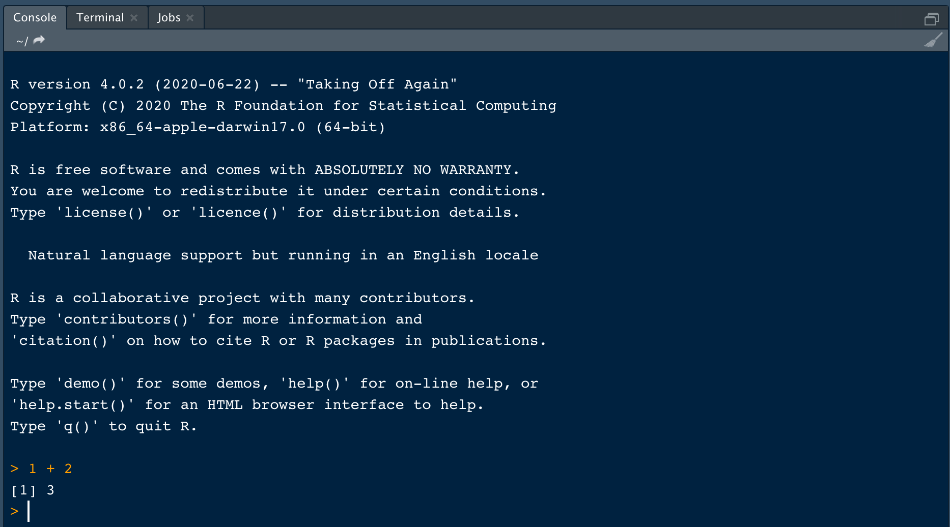
We tin can store the output of this command as a variable. Here, nosotros've named our variable result:

            effect <- 1 + two          

The <- is called the assignment operator. This operator assigns values to variables. The command higher up is translated into a sentence as:

> The effect variable gets the value of ane plus two.

One nice feature from RStudio is the keyboard shortcut for typing the consignment operator <-:

• Mac OS Ten: Option + -
• Windows/Linux: Alt + -

We highly recommend that you lot memorize this keyboard shortcut because it saves a lot of time in the long run!

When we blazon effect into the console and hitting enter, we run into the stored value of 3:

            > result <- ane + two > result [1] 3          

When we create a variable in RStudio, it saves information technology every bit an object in the R global surround. We'll discuss the surroundings and how to view objects stored in the environment in the next section.

five. The Global Environment

We tin can think of the global environment as our workspace. During a programming session in R, any variables nosotros define, or data nosotros import and save in a dataframe, are stored in our global environment. In RStudio, we tin can encounter the objects in our global environment in the Environment tab at the top right of the interface:

Nosotros'll see whatever objects we created, such every bit result, under values in the Environment tab. Notice that the value, 3, stored in the variable is displayed.

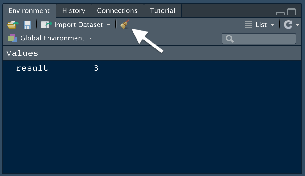
Sometimes, having too many named objects in the global environment creates defoliation. Perhaps we'd like to remove all or some of the objects. To remove all objects, click the broom icon at the top of the window:

To remove selected objects from the workspace, select the Grid view from the dropdown carte:

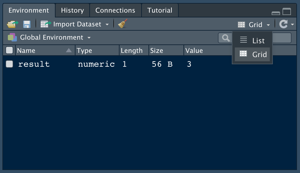
Hither we can check the boxes of the objects we'd like to remove and employ the broom icon to clear them from our Global Environment.

6. Install the tidyverse Packages

Much of the functionality in R comes from using packages. Packages are shareable collections of code, information, and documentation. Packages are substantially extensions, or add-ons, to the R program that we installed above.

I of the almost pop collection of packages in R is known as the "tidyverse". The tidyverse is a collection of R packages designed for working with data. The tidyverse packages share a common design philosophy, grammar, and information structures. Tidyverse packages "play well together". The tidyverse enables you lot to spend less time cleaning information then that y'all can focus more on analyzing, visualizing, and modeling data.

Let'southward learn how to install the tidyverse packages. The most common "cadre" tidyverse packages are:

• readr, for data import.
• ggplot2, for data visualization.
• dplyr, for data manipulation.
• tidyr, for data tidying.
• purrr, for functional programming.
• tibble, for tibbles, a modernistic re-imagining of dataframes.
• stringr, for cord manipulation.
• forcats, for working with factors (categorical information).

To install packages in R we use the congenital-in install.packages() part. We could install the packages listed above i-by-ane, only fortunately the creators of the tidyverse provide a manner to install all these packages from a single command. Type the following control in the Console and hit the enter central.

            install.packages("tidyverse")          

The install.packages() command only needs to be used to download and install packages for the first time.

seven. Load the tidyverse Packages into Retentiveness

After a package is installed on a computer'south hard drive, the library() command is used to load a package into memory:

            library(readr) library(ggplot2)          

Loading the package into memory with library() makes the functionality of a given package bachelor for utilize in the current R session. It is common for R users to have hundreds of R packages installed on their hard drive, then it would be inefficient to load all packages at once. Instead, we specify the R packages needed for a detail projection or task.

Fortunately, the cadre tidyverse packages tin can be loaded into memory with a single command. This is how the command and the output looks in the console:

            library(tidyverse)## ── Attaching packages ───────────────────────────────────────────────── tidyverse 1.iii.0 ──## ✓ ggplot2 3.iii.two ✓ purrr 0.3.four ## ✓ tibble three.0.three ✓ dplyr 1.0.0 ## ✓ tidyr 1.1.0 ✓ stringr one.iv.0 ## ✓ readr 1.3.1 ✓ forcats 0.v.0## ── Conflicts ──────────────────────────────────────────────────── tidyverse_conflicts() ── ## ten dplyr::filter() masks stats::filter() ## x dplyr::lag() masks stats::lag()          

The Attaching packages department of the output specifies the packages and their versions loaded into memory. The Conflicts section specifies any function names included in the packages that we merely loaded to memory that share the aforementioned name equally a office already loaded into memory. Using the example higher up, at present if we phone call the filter() role, R will use the code specified for this function from the dplyr package. These conflicts are generally not a problem, just information technology's worth reading the output bulletin to be certain.

8. Identify Loaded Packages

If we need to bank check which packages we loaded, we can refer to the Packages tab in the window at the lesser correct of the console.

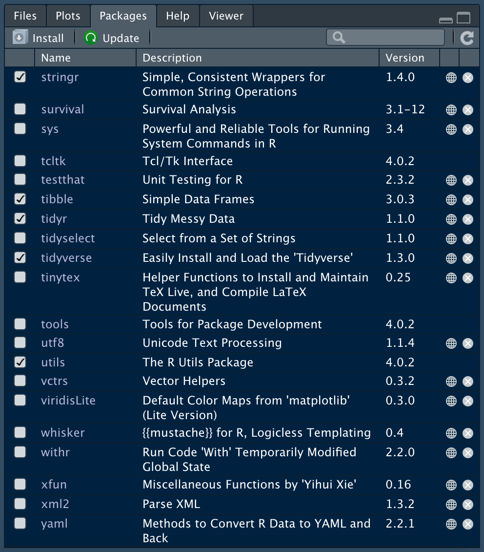
We tin can search for packages, and checking the box adjacent to a package loads information technology (the code appears in the panel).

Alternatively, entering this code into the console will display all packages currently loaded into memory:

            (.packages())          

Which returns:

            [1] "forcats" "stringr" "dplyr" "purrr" "tidyr" "tibble" "tidyverse" [8] "ggplot2" "readr" "stats" "graphics" "grDevices" "utils" "datasets"  [15] "methods" "base"          

Some other useful part for returning the names of packages currently loaded into memory is search():

            > search()  [1] ".GlobalEnv" "package:forcats" "package:stringr" "package:dplyr"   [5] "parcel:purrr" "package:readr" "package:tidyr" "bundle:tibble"   [9] "parcel:ggplot2" "bundle:tidyverse" "tools:rstudio" "package:stats"  [thirteen] "packet:graphics" "package:grDevices" "package:utils" "package:datasets"  [17] "bundle:methods" "Autoloads" "package:base"          

9. Become Help on a Bundle

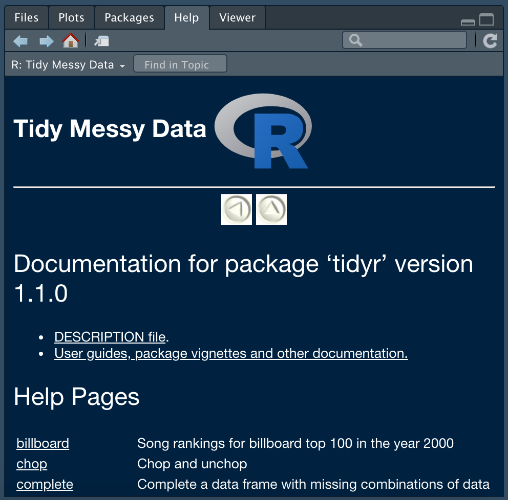
We've learned how to install and load packages. But what if nosotros'd like to acquire more about a package that we've installed? That's easy! Clicking the package name in the Packages tab takes us to the Aid tab for the selected parcel. Here's what we run into if we click the tidyr package:

Alternatively, we can blazon this command into the console and reach the same outcome:

            help(package = "tidyr")          

The help page for a package provides quick access to documentation for each function included in a packet. From the main assistance page for a bundle you can as well access "vignettes" when they are available. Vignettes provide brief introductions, tutorials, or other reference information near a package, or how to use specific functions in a package.

            vignette(packet = "tidyr")          

Which results in this list of available options:

            Vignettes in package 'tidyr':nest nest (source, html) pin Pivoting (source, html) programming Programming with tidyr (source, html) rectangle rectangling (source, html) tidy-data Tidy data (source, html) in-packages Usage and migration (source, html)          

From at that place, we can select a particular vignette to view:

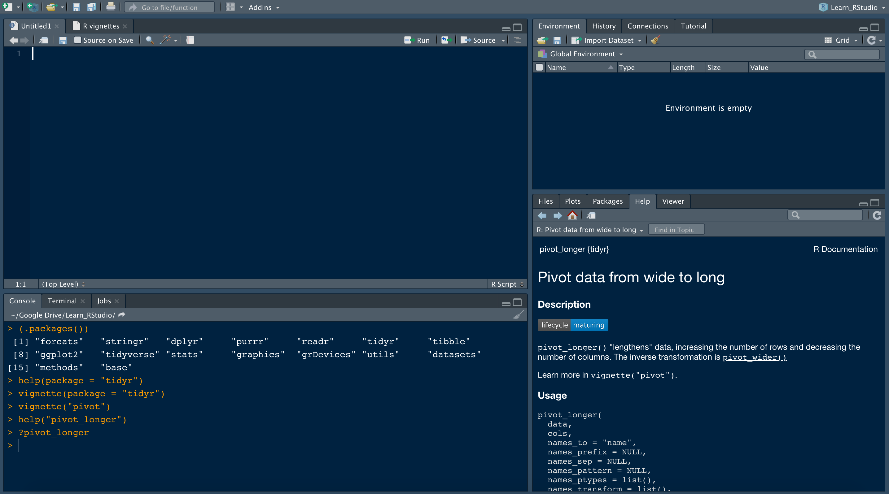
            vignette("pivot")          

Now we encounter the Pivot vignette is displayed in the Help tab. This is 1 example of why RStudio is a powerful tool for programming in R. We can access function and package documentation and tutorials without leaving RStudio!

ten. Get Assistance on a Role

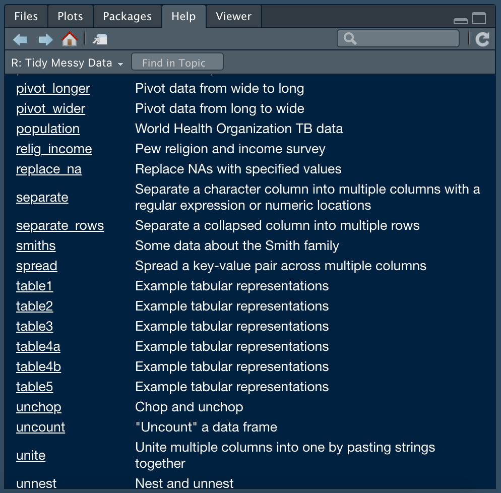
Equally we learned in the concluding section, we tin can become help on a function past clicking the package proper noun in Packages and then click on a function name to see the assistance file. Here we see the pivot_longer() function from the tidyr package is at the meridian of this list:

And if we click on "pivot_longer" we go this: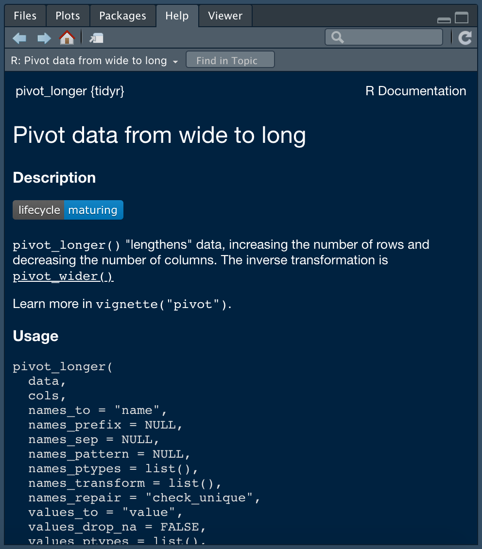

Nosotros can accomplish the same results in the Panel with any of these function calls:

            help("pivot_longer") help(pivot_longer) ?pivot_longer          

Notation that the specific Aid tab for the pivot_longer() function (or whatever function we're interested in) may not be the default result if the package that contains the role is non loaded into memory notwithstanding. In general information technology'southward all-time to ensure a specific package is loaded earlier seeking help on a office.

xi. RStudio Projects

RStudio offers a powerful feature to keep yous organized; Projects. Information technology is important to stay organized when you work on multiple analyses. Projects from RStudio let you to go on all of your important work in i identify, including code scripts, plots, figures, results, and datasets.

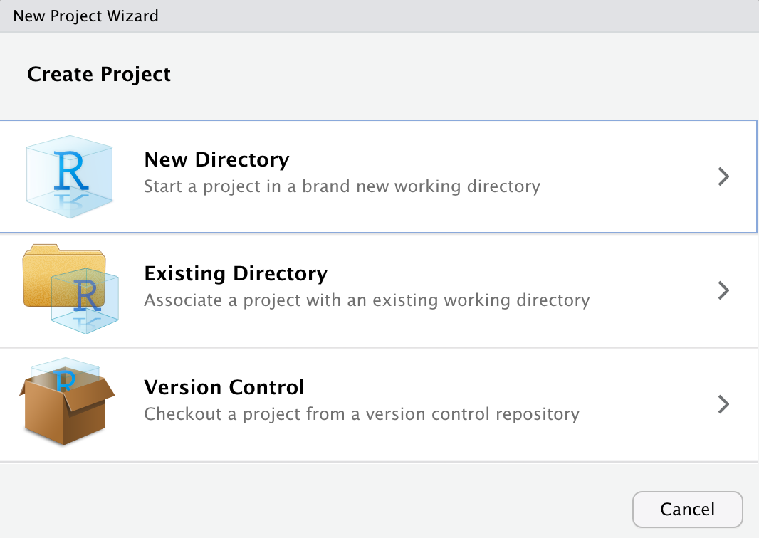
Create a new project by navigating to the File tab in RStudio and select New Project.... Then specify if yous would similar to create the project in a new directory, or in an existing directory. Here we select "New Directory":

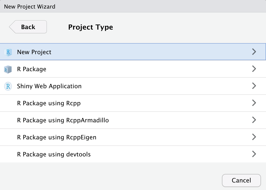
RStudio offers dedicated project types if you are working on an R package, or a Shiny Web Application. Here we select "New Project", which creates an R project:

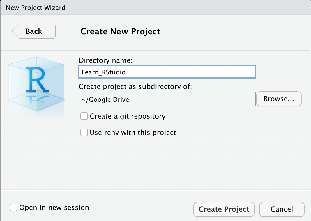
Side by side, we give our projection a name. "Create project every bit a subdirectory of:" is showing where the folder will live on the calculator. If we corroborate of the location select "Create Project", if we practise not, select "Scan" and choose the location on the reckoner where this projection folder should live.

Now in RStudio we see the name of the projection is indicated in the upper-right corner of the screen. We also see the .Rproj file in the Files tab. Any files we add to, or generate-within, this project volition appear in the Files tab.

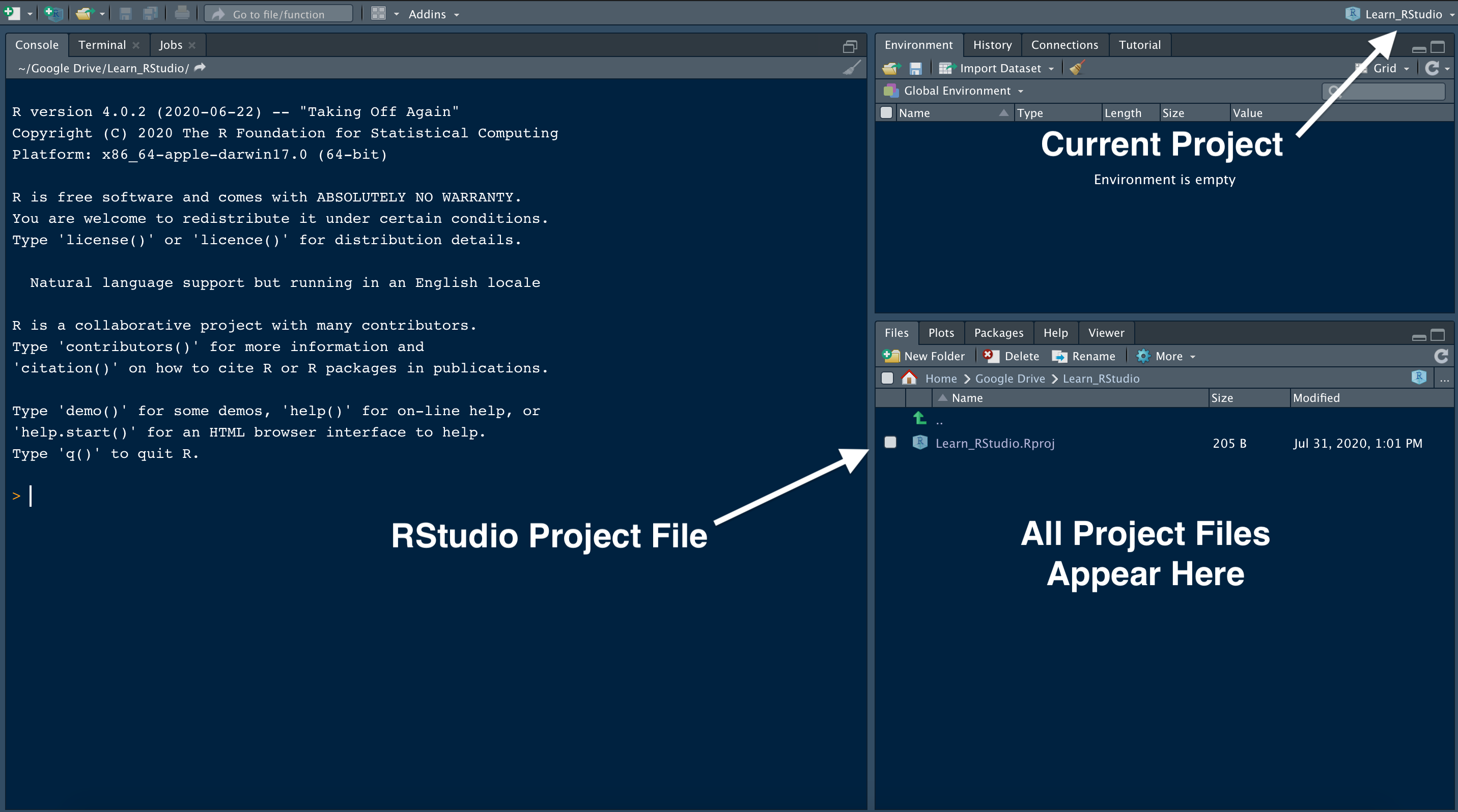
RStudio Projects are useful when you need to share your work with colleagues. You can send your project file (catastrophe in .Rproj) along with all supporting files, which volition go far easier for your colleagues to recreate the working environs and reproduce the results.

12. Save Your "Real" Work. Delete the Rest.

This tip comes from our 23 RStudio Tips, Tricks, and Shortcuts blog post, but it'south so important that we are sharing information technology here besides!

Do good housekeeping to avoid unforeseen challenges downwards the road. If you lot create an R object worth saving, capture the R code that generated the object in an R script file. Save the R script, simply don't salve the environment, or workspace, where the object was created.

To prevent RStudio from saving your workspace, open Preferences > General and un-select the selection to restore .RData into workspace at startup. Be sure to specify that you lot never desire to relieve your workspace, similar this:

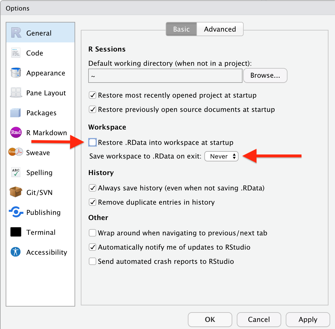
At present, each time you open RStudio, you lot will begin with an empty session. None of the code generated from your previous sessions volition be remembered. The R script and datasets tin be used to recreate the surroundings from scratch.

Other experts concur that not saving your workspace is best do when using RStudio.

thirteen. R Scripts

As we worked through this tutorial, we wrote code in the Panel. As our projects become more circuitous, nosotros write longer blocks of code. If we want to save our work, it is necessary to organize our code into a script. This allows us to keep rail of our work on a project, write make clean code with plenty of notes, reproduce our work, and share information technology with others.

In RStudio, nosotros tin write scripts in the text editor window at the meridian left of the interface:

To create a new script, we can use the commands in the file carte du jour:

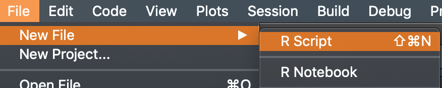
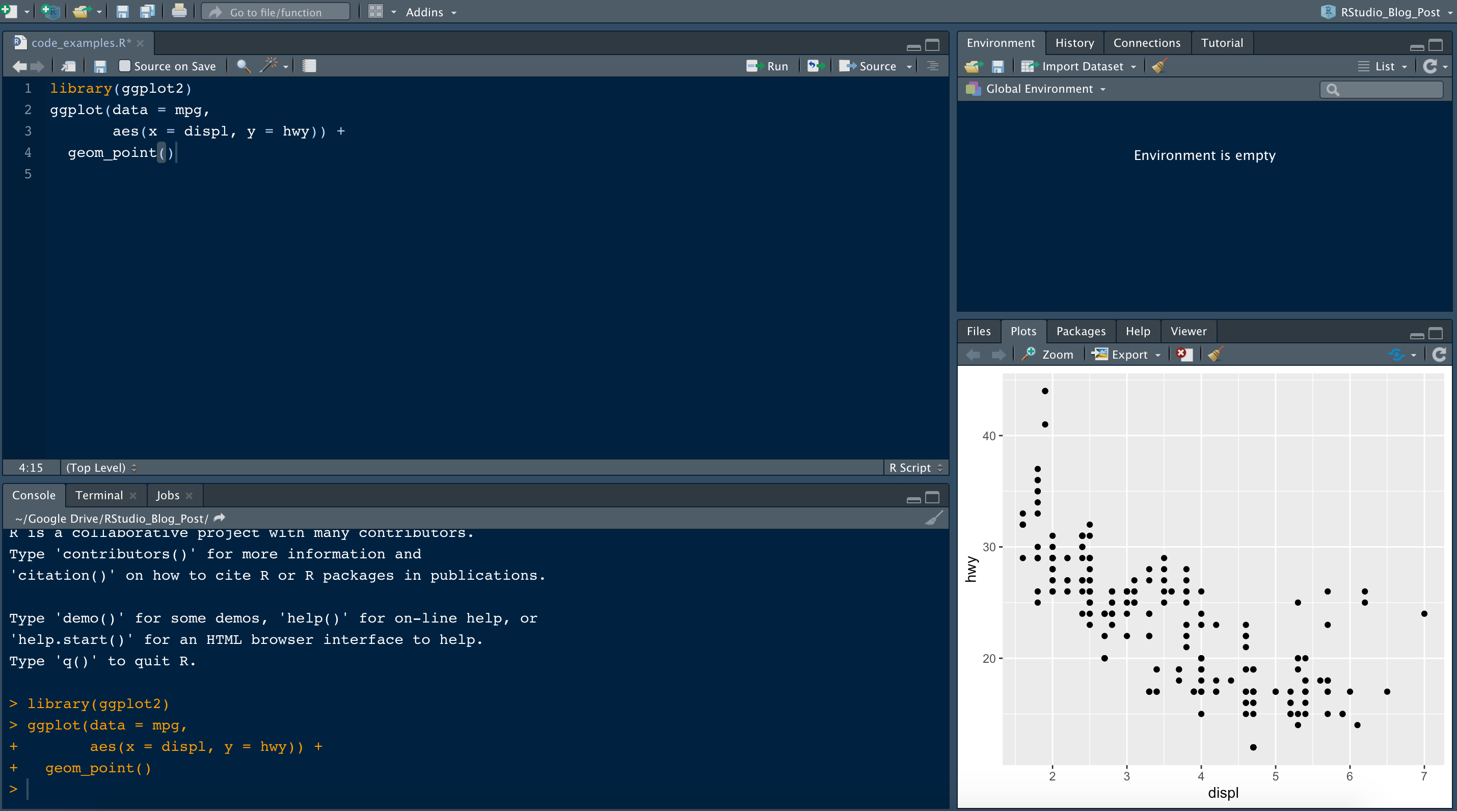
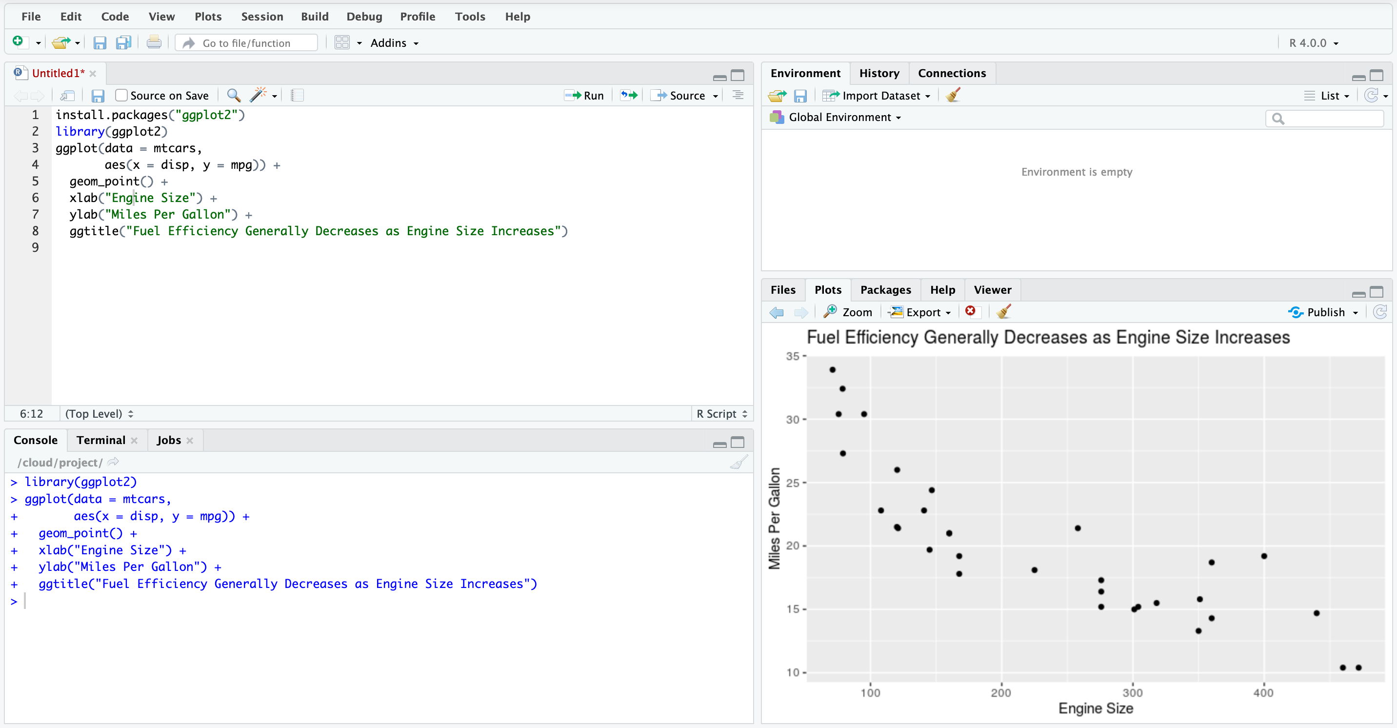
Nosotros can also utilize the keyboard shortcut Ctrl + Shift + Northward. When we save a script, information technology has the file extension .R. As an example, we'll create a new script that includes this code to generate a scatterplot:

            library(ggplot2) ggplot(data = mpg,        aes(x = displ, y = hwy)) +   geom_point()          

To save our script we navigate to the File bill of fare tab and select Save. Or nosotros enter the following command:

• Mac OS 10: Cmd + Due south
• Windows/Linux: Ctrl + S

14. Run Code

To run a unmarried line of code nosotros typed into our script, nosotros can either click Run at the top right of the script, or employ the following keyboard commands when our cursor is on the line nosotros want to run:

• Mac OS X: Cmd + Enter
• Windows/Linux: Ctrl + Enter

In this case, nosotros'll demand to highlight multiple lines of code to generate the scatterplot. To highlight and run all lines of lawmaking in a script enter:

• Mac OS Ten: Cmd + A + Enter
• Windows/Linux: Ctrl + A + Enter

Let's check out the result when we run the lines of code specified above:

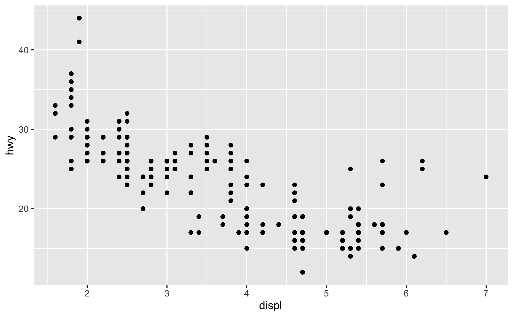
Side annotation: this scatterplot is generated using data from the mpg dataset that is included in the ggplot2 package. The dataset contains fuel economy data from 1999 to 2008, for 38 popular models of cars.

In this plot, the engine displacement (i.e. size) is depicted on the 10-axis (horizontal centrality). The y-centrality (vertical axis) depicts the fuel efficiency in miles-per-gallon. In general, fuel economy decreases with the increment in engine size. This plot was generated with the tidyverse package ggplot2. This package is very pop for data visualization in R.

15. Admission Built-in Datasets

Want to larn more about the mpg dataset from the ggplot2 package that we mentioned in the last example? Do this with the following command:

            data(mpg, packet = "ggplot2")          

From there yous can take a look at the commencement six rows of data with the head() function:

            head(mpg)          

            ## # A tibble: 6 10 11 ##   manufacturer model displ  twelvemonth   cyl trans      drv     cty   hwy fl    class  ##                           ## 1 audi         a4      1.8  1999     4 car(l5)   f        18    29 p     compa… ## 2 audi         a4      1.viii  1999     four transmission(m5) f        21    29 p     compa… ## three audi         a4      2    2008     iv manual(m6) f        xx    31 p     compa… ## 4 audi         a4      2    2008     iv automobile(av)   f        21    30 p     compa… ## 5 audi         a4      2.eight  1999     6 auto(l5)   f        16    26 p     compa… ## half dozen audi         a4      2.viii  1999     six manual(m5) f        eighteen    26 p     compa…          

Obtain summary statistics with the summary() role:

            summary(mpg)          

            ##  manufacturer          model               displ            year      ##  Length:234         Length:234         Min.   :1.600   Min.   :1999   ##  Course :character   Class :character   1st Qu.:2.400   1st Qu.:1999   ##  Manner  :character   Style  :character   Median :3.300   Median :2004   ##                                        Hateful   :three.472   Mean   :2004   ##                                        3rd Qu.:4.600   3rd Qu.:2008   ##                                        Max.   :7.000   Max.   :2008   ##       cyl           trans               drv                 cty        ##  Min.   :4.000   Length:234         Length:234         Min.   : 9.00   ##  1st Qu.:four.000   Class :graphic symbol   Class :graphic symbol   1st Qu.:14.00   ##  Median :vi.000   Mode  :grapheme   Style  :character   Median :17.00   ##  Mean   :5.889                                         Mean   :16.86   ##  3rd Qu.:8.000                                         3rd Qu.:19.00   ##  Max.   :8.000                                         Max.   :35.00   ##       hwy             fl               grade           ##  Min.   :12.00   Length:234         Length:234         ##  1st Qu.:xviii.00   Class :character   Class :character   ##  Median :24.00   Mode  :character   Mode  :character   ##  Mean   :23.44                                         ##  3rd Qu.:27.00                                         ##  Max.   :44.00          

Or open the help page in the Help tab, like this:

            help(mpg)          

Finally, at that place are many datasets built-in to R that are ready to work with. Built-in datasets are handy for practicing new R skills without searching for information. View available datasets with this command:

            data()          

16. Style

When writing an R script, it's skilful exercise to specify packages to load at the top of the script:

            library(ggplot2)          

Every bit nosotros write R scripts, it's besides good practice add together comments to explain our lawmaking (# like this). R ignores lines of code that begin with #. Information technology's common to share code with colleagues and collaborators. Ensuring they empathize our methods volition be very important. Only more importantly, thorough notes are helpful to your future-self, so that you tin sympathise your methods when you revisit the script in the hereafter!

Here'south an example of what comments look like with our scatterplot code:

            library(ggplot2)  # fuel economy data from 1999 to 2008, for 38 popular models of cars # engine deportation (size) is depicted on the x-centrality # fuel efficiency is depicted on the y-centrality ggplot(data = mpg,        aes(x = displ, y = hwy)) +   geom_point()          

17. Reproducible Reports with R Markdown

The comments used in the example to a higher place are fine for providing cursory notes nearly our R script, merely this format is not suitable for authoring reports where we need to summarize results and findings. Nosotros can author nicely formatted reports in RStudio using R Markdown files.

R Markdown is an open-source tool for producing reproducible reports in R. R Markdown enables us to keep all of our code, results, and writing, in one place. With R Markdown we accept the option to export our work to numerous formats including PDF, Microsoft Word, a slideshow, or an html certificate for employ in a website.

If you would like to learn R Markdown, check out these Dataquest blog posts:

• Getting Started with R Markdown — Guide and Cheatsheet
• R Markdown Tips, Tricks, and Shortcuts

18. Employ RStudio Deject

RStudio at present offers a cloud-based version of RStudio Desktop called RStudio Cloud. RStudio Cloud allows you to lawmaking in RStudio without installing software, you merely need a spider web browser. Almost everything nosotros've learned in this tutorial applies to RStudio Deject!

Work in RStudio Cloud is organized into projects similar to the desktop version. RStudio Cloud enables yous to specify the version of R you wish to use for each projection. This is great if yous are revisiting an older project built around a previous version of R.

RStudio Cloud as well makes it easy and secure to share projects with colleagues, and ensures that the working environment is fully reproducible every time the project is accessed.

The layout of RStudio Deject is very similar to RStudio Desktop:

nineteen. Go Your Easily Dirty!

The all-time way to learn RStudio is to use what we've covered in this tutorial. Jump in on your own and familiarize yourself with RStudio! Create your own projects, save your work, and share your results. Nosotros can't emphasize the importance of this plenty.

Not certain where to start? Check out the boosted resources listed below!

Additional Resources

If you enjoyed this tutorial, come learn with the states at Dataquest! If you are new to R and RStudio, we recommend starting with the Dataquest Introduction to Information Analysis in R form. This is the commencement course in the Dataquest Information Analyst in R path.

For more advanced RStudio tips check out the Dataquest blog post 23 RStudio Tips, Tricks, and Shortcuts.

Learn how to load and make clean data with tidyverse tools in this Dataquest weblog mail service.

RStudio has published numerous in-depth how to articles about using RStudio. Observe them here.

At that place is an official RStudio Weblog.

If yous would similar to acquire R Markdown, check out these Dataquest blog posts:

• Getting Started with R Markdown — Guide and Cheatsheet
• R Markdown Tips, Tricks, and Shortcuts

Larn R and the tidyverse with R for Data Science by Hadley Wickham. Solidify your knowledge past working through the exercises in RStudio and saving your work for future reference.

Bonus: Cheatsheets

RStudio has published numerous cheatsheets for working with R, including a detailed cheatsheet on using RStudio! Select cheatsheets can be accessed from inside RStudio by selecting Assist > Cheatsheets.

Ready to level upwardly your R skills?

Our Data Annotator in R path covers all the skills y'all demand to state a job, including:

• Data visualization with ggplot2
• Avant-garde information cleaning skills with tidyverse packages
• Important SQL skills for R users
• Fundamentals in statistics and probability
• ...and much more than

There's nothing to install, no prerequisites, and no schedule.

Tags

Source: https://www.dataquest.io/blog/tutorial-getting-started-with-r-and-rstudio/

Posted by: byrdthany1971.blogspot.com

Share this post